When building analytics on top of a relational datbase like Postgres, MySQL, Sql Server or Oracle, star schemas can be useful at various points in the data model. In this article I’m going to build a simple analytics schema starting from a CSV file, and transforming the data into a simple star schema with two dimension tables.

I am going to use Postgres 11 for the database, and Tweakstreet preview build 27 as the ETL tool. Both are freely available for download if you wish to follow along.

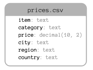
Our sample data contains worldwide dollar-equivalent pricing of certain supermarket goods. A single source CSV file contains observations of prices for supermarket goods as seen in a certain region.

The source file contains data like this:

All data is artificially generated. The sample files are available for download: input_full.csv.zip 1,000,000 records input file — ca. 3MB zipped

When loading this data into a relational database for analytics, we want to keep all information, but avoid duplication. The aim is to keep storage footprint low, and query performance high.

I want to treat the price field as a fact measure that I can average over locations or products. I split the item and location attributes into dimension tables.

One benefit of this design is that location fields and item fields are each going to have a relatively small amount of combinations compared with the total amount of observations. This will keep the dimension tables small and efficient to join to the fact table if needed.

Dimension tables that consist of a dynamic combination of fields with no historization mechanism are sometimes called junk dimensions. They often consist of left-over fields that remain after all other dimension tables have been modeled, hence the term junk dimensions.

In a real-world scenario, the date — and possibly time — of the observation would be another crucial piece of information. It would be modeled as a key into the date dimension table. Additionally, a real-world scenario would include house-keeping fields on all tables, such as a load_id, load_date, or last_updated columns. I am going to omit these aspects in this article, to avoid distractions.

Once the model and data are in place we’d like to query it. A typical analytical query would retrieve some ranking based on measures, grouped by attributes. The following query retrieves the top 10 countries with the cheapest average price for waffles:

Once all data is loaded, the result returns a corresponding list:

Most analytics, OLAP, and reporting tools understand the concept of star schemas — that is fact tables containing measures that are connected to any number of dimension tables through foreign keys — and let you quickly formulate analytical queries like this through their graphical user interface.

For Postgres 11 the following SQL creates the tables and lookup indexes for the data model:

Tweakstreet can generate the necessary SQL when configuring the steps that work with database tables.

There are two basic approaches to loading fact and dimension tables:

• inline: populate dimension tables as part of the fact loading process
• tiered: populate all dimensions first, populate all fact tables second

The tiered approach has many benefits. It offers better concurrency properties — please note that the dimension tables are not directly related, so they can be loaded in parallel. It also has good recovery options when technical errors occur: if the dimension loading stage completes successfully, you know that you don’t need to repeat it when recovering from errors during fact loading.

The downside of the tiered approach is that you need to process input data multiple times. Once to fill the dimensions, and another time to load the facts.

For the sake of simplicity, I am going to use the inline loading approach and load the dimensions and facts in a single data flow. In any non-trivial scenario with shared dimension tables, I would recommend using the tiered approach instead.

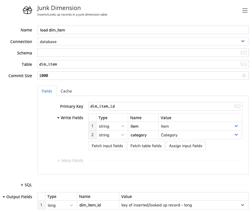
I am going to use the Junk Dimension step of Tweakstreet to load the dimension tables. The step needs configuration mapping input fields to database tables. It takes care of loading the dimension table efficiently.

The step needs to know the database connection to work with, the table to use, and the fields to use. It returns the primary key of the dimension record corresponding to the configured write fields.

If we had any housekeeping fields like load_id, load_date etc. they would go into the meta fields section, which contains fields that are not part of the lookup, but they are inserted in case a corresponding record is not in the table yet.

For every input record the step performs the following operations:

Following this process, the step returns the primary key for a corresponding dimension record for every input record.

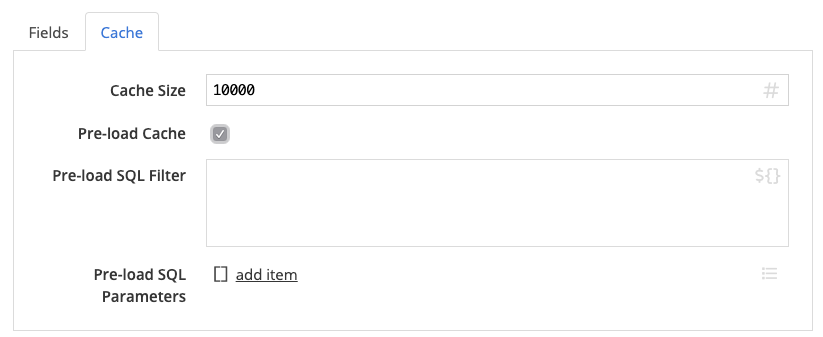
The cache plays an important role in the efficient execution of the step. You can configure how many data rows are kept in cache, and whether it is pre-loaded with data from the database table at the beginning of the process. Every cache-hit reduces the amount of round-trips to the database. Ideally you can make the cache big enough to fit all records in-memory.

For cases where the entire dimension is too large to fit into memory, the step gives you control over which records to initialize the cache with. You can supply a WHERE clause to the cache population query. If you have information about incoming data, such as that based on its source, some fields are likely to be constant, you can use that knowledge to initialize the cache efficiently.

The flow begins by re-creating the fact table. Usually you’d add to fact tables, but this one is a snapshot table we want to re-populate on every run. Next the flow is reading the source fields using the CSV input step. It proceeds to load the dim_item and dim_location tables using the Junk Dimension step, retrieving the keys of the corresponding dimension records. As a final step, the SQL Insert step is used to insert the fact records into the database.

The flow executes all steps in parallel. The read file step reads records from the input file and passes them on to a queue connected to the next step. This way, only a small set of records is in memory at any given time, and the whole process can load millions of records efficiently.

When constructing the data flow, you can execute it at any time, and follow the evolution of the data in your stream. The following screencast shows the entire process of interactively constructing the loading process from scratch, with an example of how to execute it from the command line.

In case you want to follow along, download Tweakstreet, and make sure to drop the Postgres JDBC driver into your $HOME/.tweakstreet/drivers folder as described in the configuration documentation. I am using preview build 0.0.27 during this video.

You can run Tweakstreet flows through the command line, making it easy to schedule runs using the scheduling software of choice for your OS.

For example, on my mac, I can run the flow by invoking /Applications/Tweakstreet.app/Contents/bin/engine.sh like this:

Check the command line docs for instructions to run on Linux and Windows.